


Next: Dynamical system, a description
Up: Applications of recurrence quantified
Previous: Applications of recurrence quantified
Recurrence Plot (RP) was initially introduced by Eckman et al. (1987)
[1]
as a tool for analyzing experimental time series data, especially useful
for finding hidden correlations in highly complicated data and to determine the
stationarity of the time series. This method allows the identification of system
properties that cannot be observed by the linear and nonlinear usual approaches
It is worthwhile mentioning the simplicity of the algorithms during numerical
calculations too.
An RP is an injective application of a single reconstructed trajectory to the
boolean matrix space, each pair  ,
,  coming from the time series is
related with a pair
coming from the time series is
related with a pair  , called recurrence points.
Let us consider
, called recurrence points.
Let us consider  values of a time series given by
 ,
with large enough in order to evaluate the embedding dimension by using
the false nearest neighbor [2]
(
,
with large enough in order to evaluate the embedding dimension by using
the false nearest neighbor [2]
( ) and the time delay (
 )
by looking at the relative minimum in the mutual information [3]
Following Takens' embedding theorem [4],
the dynamics can be appropriately represented
by the phase space trajectory reconstructed by using the time delay vectors
)
by looking at the relative minimum in the mutual information [3]
Following Takens' embedding theorem [4],
the dynamics can be appropriately represented
by the phase space trajectory reconstructed by using the time delay vectors
 .
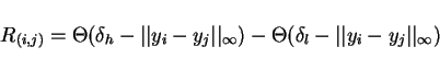
and the recurrence matrix is:
.
and the recurrence matrix is:
 |
(1) |
where  is the Heaviside function and the matrix is symmetric.
This means a RP is built by comparing
all delayed vectors with each other. A dark dot is plotted, (
is the Heaviside function and the matrix is symmetric.
This means a RP is built by comparing
all delayed vectors with each other. A dark dot is plotted, ( ) with
integer coordinates when
) with
integer coordinates when
 ,
otherwise a white dot is plotted (
,
otherwise a white dot is plotted ( ).
The interval
).
The interval
![$[\delta_l, \delta_h]$](img19.png) it is known as threshold corridor.
The choice of this interval is critical,if too large produces a saturation
of the RP including irrelevant points, and if too narrow loses information.
Since up to now in the literature there is no satisfactory solution,
an educated guess should be appropriate.
Webber and Zbilut[15] prescribe a threshold corridor corresponding to lower
ten percent of the entire distance range in the corresponging
unthresholded recurrence plot.
In this work we use
it is known as threshold corridor.
The choice of this interval is critical,if too large produces a saturation
of the RP including irrelevant points, and if too narrow loses information.
Since up to now in the literature there is no satisfactory solution,
an educated guess should be appropriate.
Webber and Zbilut[15] prescribe a threshold corridor corresponding to lower
ten percent of the entire distance range in the corresponging
unthresholded recurrence plot.
In this work we use
![$[\sigma/10^5, \sigma/10^2]$](img20.png) , where
, where  is the
standard deviation.
Webber et al. [5] in order to characterize and analyze recurrent plots
introduced a set of quantifiers, which are collectively called
recurrence quantified analysis (RQA). The first of this quantifiers
is the % recurrence (%REC), defined as:
is the
standard deviation.
Webber et al. [5] in order to characterize and analyze recurrent plots
introduced a set of quantifiers, which are collectively called
recurrence quantified analysis (RQA). The first of this quantifiers
is the % recurrence (%REC), defined as:
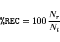 |
(2) |
where
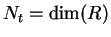 (every possible points)
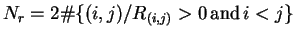
and
(every possible points)
and  is number of recursive points given by:
 The slope of the linear region in the S-shaped %REC vs. corridor width
is the correlation dimension. The second RQA quantifier
is called % determinism (%DET); and it is defined as:
The slope of the linear region in the S-shaped %REC vs. corridor width
is the correlation dimension. The second RQA quantifier
is called % determinism (%DET); and it is defined as:
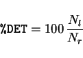 |
(3) |
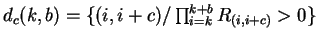
where  is called the number of periodic dots given by:
 and a periodic line with length
  , origin
  and zone
  is defined as:
 The %DET is related with the organization of the RP.
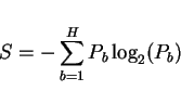
The third RQA quantifier, called entropy (S), is closely related to %DET.
The %DET is related with the organization of the RP.
The third RQA quantifier, called entropy (S), is closely related to %DET.
 |
(4) |
where  is the length of the maximum periodic line,
 is the relative frequency of the periodic lines with length
  .
The label entropy is just that, a label, not to be confused with Shannon's
entropy since there is not a one to one correspondence between this quantifier
and the Shannon's entropy. This quantity should be labeled more properly as
first rate cumulant since it is related with the relative frequency
fluctuations.
Moreover, for periodic orbits they are mapped onto diagonals with
different lengths and uniformly distributed, giving values of
.
The label entropy is just that, a label, not to be confused with Shannon's
entropy since there is not a one to one correspondence between this quantifier
and the Shannon's entropy. This quantity should be labeled more properly as
first rate cumulant since it is related with the relative frequency
fluctuations.
Moreover, for periodic orbits they are mapped onto diagonals with
different lengths and uniformly distributed, giving values of  , with a maximum
value.
Webber assumes that
, with a maximum
value.
Webber assumes that  is related with
Shannon's entropy if and only if the system is chaotic and the embedding dimension
large enough.
The fourth quantifier is the longest periodic line found during the computation
of %DET given by the
is related with
Shannon's entropy if and only if the system is chaotic and the embedding dimension
large enough.
The fourth quantifier is the longest periodic line found during the computation
of %DET given by the
 .
Eckman et al. claim that line lengths on RP are directly related to
inverse of the largest positive Lyapunov exponent.
Short lines values are therefore indicative of chaotic or stochastic behavior.
.
Eckman et al. claim that line lengths on RP are directly related to
inverse of the largest positive Lyapunov exponent.
Short lines values are therefore indicative of chaotic or stochastic behavior.
Next: Dynamical system, a description
Up: Applications of recurrence quantified
Previous: Applications of recurrence quantified
Horacio Castellini
2004-10-27